WRF-Hydro® FAQ's
Frequently Asked Questions
Below are some highlights. Version 5.2.0 of the Community WRF-Hydro® source code is consistent with the NOAA National Water Model (NWM) v2.1 code in operations plus the following additions and fixes:
- Added snow-related vars to retrospective output configuration
- Added SFCFRNOFF output flag tied to overland runoff switch
- Support GNU Fortran version 10.x and 11.x
- Added missing crop and soil NoahMP namelist options
- Removed deprecated namelist options for Reach-Lakes configuration
- Fixed issues with using gridded domains with very small dimensions
- Added ISLAKE mask flag to relevant NoahMP code
- Updated NUOPC cap component with improved MPI support and to read and write restarts
- Updated default channel parameters for gridded configuration
- Performance improvements to channel network initialization
- Added global title attribute to all output netCDF files
- Updated namelist templates
Version 5.2 Citation is as follows:
- Gochis, D.J., M. Barlage, R. Cabell, M. Casali, A. Dugger, K. FitzGerald, M. McAllister, J. McCreight, A. RafieeiNasab, L. Read, K. Sampson, D. Yates, Y. Zhang (2020). The WRF-Hydro® modeling system technical description, (Version 5.1.1). NCAR Technical Note. 108 pages. Available online at:https://ral.ucar.edu/sites/default/files/public/projects/wrf-hydro/tech…
Version 5.1.1 Citation is as follows:
- Gochis, D.J., M. Barlage, R. Cabell, M. Casali, A. Dugger, K. FitzGerald, M. McAllister, J. McCreight, A. RafieeiNasab, L. Read, K. Sampson, D. Yates, Y. Zhang (2020). The WRF-Hydro® modeling system technical description, (Version 5.1.1). NCAR Technical Note. 107 pages. Available online at: https://ral.ucar.edu/sites/default/files/public/WRFHydroV511TechnicalDe… Source Code DOI:10.5281/zenodo.3625238
Version 5.0 and 5.0.3 Citation is as follows:
- Gochis, D.J., M. Barlage, A. Dugger, K. FitzGerald, L. Karsten, M. McAllister, J. McCreight, J. Mills, A. RafieeiNasab, L. Read, K. Sampson, D. Yates, W. Yu, (2018). The WRF-Hydro modeling system technical description, (Version 5.0). NCAR Technical Note. 107 pages. Available online at https://ral.ucar.edu/sites/default/files/public/WRFHydroV5TechnicalDesc…. Source Code DOI:10.5065/D6J38RBJ
Version 3 Citation is as follows:
- Gochis, D.J., W. Yu, D.N. Yates, 2015: The WRF-Hydro model technical description and user's guide, version 3.0. NCAR Technical Document. 123 pages. Available online at https://ral.ucar.edu/sites/default/files/public/WRF_Hydro_User_Guide_v3…. Source Code DOI:10.5065/D6DN43TQ
- A compiler. WRF-Hydro supported compilers are the Portland Group FORTRAN compiler, the Intel ‘ifort’ compiler and the public license GNU Fortran compiler ‘gfort’ (for use with Linux-based operating systems on desktops and clusters)
- MPICH or OpenMPI
- NetCDF C & Fortran Libraries - NetCDF C Version 4.4.1.1 and NetCDF F Version 4.4.4 or greater available from https://www.unidata.ucar.edu/software/netcdf/ (These libraries need to be compiled with the same compilers as you will use to compile WRF-Hydro) Note: if you are coupling with WRF, the WRF user guide instructs users to build netCDF 4 with the --disable-netcdf-4 flag. However netCDF 4 must be enabled to work with WRF-Hydro. Please check that this flag has been enabled. Information regarding linking libraries can be found in the netCDF documentation https://www.unidata.ucar.edu/software/netcdf/docs/getting_and_building_netcdf.html https://www.unidata.ucar.edu/software/netcdf/docs/building_netcdf_fortran.html
- WRF-Hydro model code which is available from https://ral.ucar.edu/projects/wrf_hydro
We are not able to cover the breadth of all possible installation configurations as they are facility and machine dependent.
WRF-Hydro requires a number of machine and distribution-specific libraries. While we are not able to cover the breadth of all possible configurations, we offer an example of dependency installation for a base Ubuntu Linux distribution to serve as a starting point for other configurations.
Example of Dependency Installation for a Base Ubuntu Linux Distribution
The example below uses the GNU compiler and MPICH libraries, and commands are issued as root user in the bash shell. Note: We can not support inquiries regarding this installation. Please discuss your unique set up with your support staff.
|
################################## ###Get libraries available through apt-get ################################## apt-get update apt-get install -wget bzip2 \ ca-certificates vim hibhdf5-dev \ gfortran g++ m4 make libswitch-perl \ ca-certificates \ git tcsh libopenmpi-dev \ libnetcdff-dev libnetcdf-dev \ netcdf-bin \ apt-get clean
################################## ###Check netCDF installs (optional) ################################## nf-config --all nc-config --all |
- We suggest you begin by downloading the model code and follow the Techincal Description and User Guides.
- Build the model and run a provided Test Case with 'idealized' forcing to assure that your set up is correct. The test case packages provide all the needed input data required for running the model over a small to moderate domain. Make sure that the test case version and model code version matches!
- Then run the test case with one of the configurations available and compare your model output with the output files provided.
- Next create customized geographical inputs and forcing data
- Run the model with your customized geographical inputs, the land surface model only, and idealized forcing
- Run the model with your customized geographical inputs, the land surface model only, and your forcing data
- Run the model with your customized geographical inputs, your forcing data, and minimal routing physics. Turn physics options on one at a time starting with 1. Sfc/subsfc 2. GW/baseflow 3. Channel flow 4. Reservoirs
- Once you finalize your configuration you can then move on to a full model simulation.
The WRF-Hydro model source code is now hosted in a GitHub repository. Please see our guidelines for contributing.
If you want to create customized geographical inputs for a specific region, below is an illustration of the workflow for creating them for running WRF-Hydro in a standalone mode. Note: this workflow only works with the Noah-MP land surface model (LSM). See the How To Build & Run WRF-Hydro In Standalone Mode document for a step by step guide.
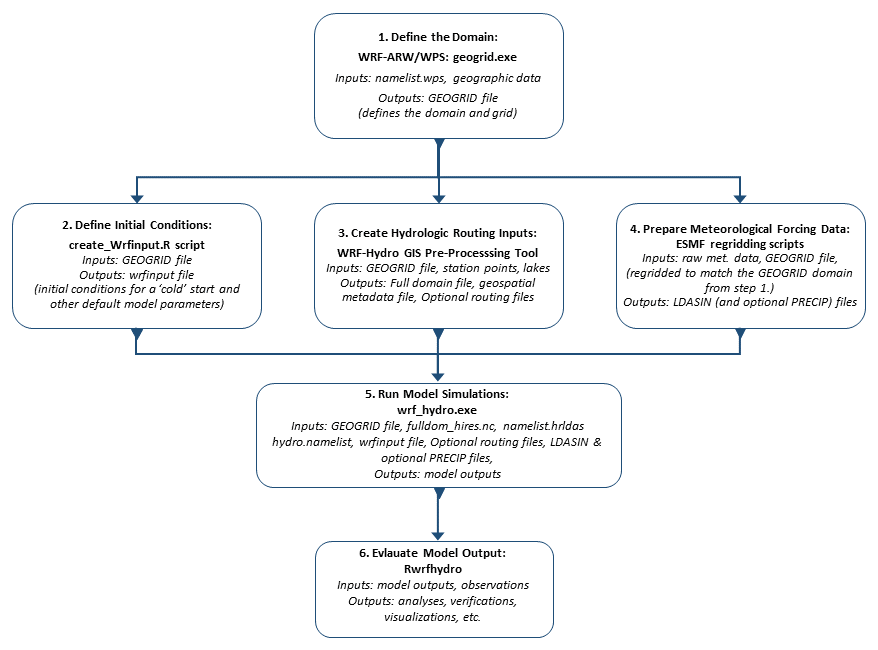
We recommend that you redo your preprocessed input files to work with the most recent version of code. All of the needed tools and scripts to create customized input have been updated to work with Version 5.1.1 and are available from our pre-processing tools and regridding scripts web pages.
We still support Noah because it is largley frozen from a development aspect. NoahMP (multiphysics parameterizations) provides a framework within the column land surface model for multiple options of process representation and thus is more extensible.
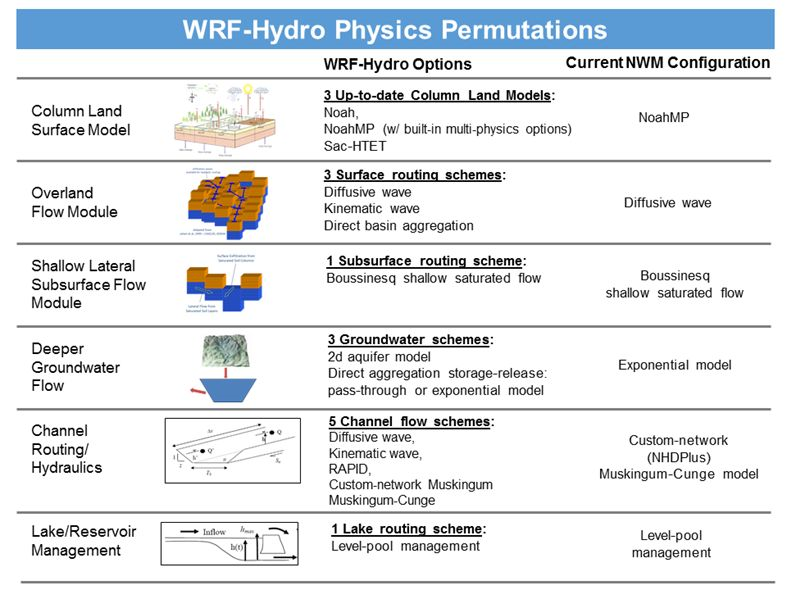
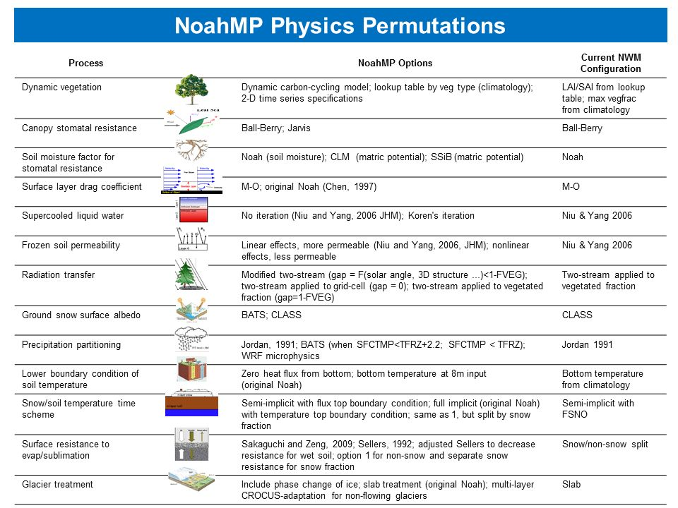 WRF-Hydro is the current modeling framework of the National Water Model (NWM). The NWM is one configuration of WRF-Hydro. The first image above illustrates the physics permutations available in WRF-Hydro and those used in the configuration of the NWM. The second image above illustrates the physics permutations available in the Noah-MP land surface model and those used in the configuration of the NWM. For more information regarding the operational configuration, input, and output data of the National Water Model see the Office of Water Prediction website: http://water.noaa.gov/about/nwm and the Open Commons Consortium Environmental Data Commons website: http://edc.occ-data.org/nwm/. The NWM/WRF-Hydro modeling system suite of tools for data preparation, evaluation, and calibration is continually under development and will be rolled out to the community as each tool becomes finalized with supporting documentation for public usage. To be notified when tools become available please subscribe to our email list.
The National Water Model v1.2 25-year retrospective simulation (Jan 1 1993 - Dec 31 2017) data is available through the Open Commons Consortium Environmental Data Commons website: http://edc.occ-data.org/nwm/. The 25 year retrospective provides historical context to current conditions and can be used to infer flow frequencies and perform temporal analyses.
Five new datasets in the AWS Public Datasets program that are tagged for sustainability and are now available in the Registry for Open Data on AWS (https://registry.opendata.aws/). Those include:
1. NOAA National Water Model Reanalysis (Onboarded by NOAA) https://registry.opendata.aws/nwm-archive/
2. NOAA National Water Model Short-Range Forecast (Onboarded by NOAA):https://registry.opendata.aws/noaa-nwm-pds/
3. NOAA Global Historical Climatology Network Daily (Onboarded by NOAA) https://registry.opendata.aws/noaa-ghcn/
4. NOAA NDFD (National Digital Forecast Database) and NDGD (National Digital Guidance Database) (Onboarded by Cornell University) https://registry.opendata.aws/cornell-eas-data-lake/
5. ECMWF ERA5 Reanalysis (Onboarded by Intertrust) https://registry.opendata.aws/ecmwf-era5/
You can explore additional datasets relevant for sustainability by visiting https://registry.opendata.aws/?search=sustainability.
The National Water Model v2.0 25-year retrospective simulation data for 'full physics' and 'long range' runs are available through the Google Cloud https://console.cloud.google.com/storage/browser/national-water-model-v2?pli=1. The 25 year retrospective provides historical context to current conditions and can be used to infer flow frequencies and perform temporal analyses.
The differences are:
- 1) Model resolution: 1-km land surface grid and 250-m terrain routing grid for “full physics” vs. 1-km land surface grid and 1-km terrain routing grid for “long range”
- 2) Subsurface routing and surface overland flow routing turned on for “full physics” but not turned on for “long range”
- 3) Terrain routing output for “full physics” vs. no terrain routing output for “long range”
We are not able to cover the breadth of all possible configurations as they are machine dependent. However, If you do not define "$NETCDF_LIB" and "$NETCDF_INC" from your environment, the configure script will use the extension from "$NETCDF/include" for $NETCDF_INC and "$NETCDF/lib" for $NETCDF_LIB. If $NETCDF is also not defined from your environment, then you will get the error message. Before you run the configure script, you can check the environment variable by typing the commands :
- echo $NETCDF
- echo $NETCDF_INC
- echo $NETCDF_LIB
Make sure either $NETCDF_INC and $NETCDF_LIB or $NETCDF are defined.
Often segmentation faults occur with WRF-Hydro when the domains for the land surface model and routing are not properly created in dimension or the hydro.namelist setting which specifies the routing grid dimension (dx) is not properly set. Other reasons one might see a segmentation fault error is when the program attempts to access a memory location that it is not allowed to access, or attempts to access a memory location in a way that is not allowed (for example, attempting to write to a read-only location or to overwrite part of the operating system). You might check every place in your program that uses pointers or subscripts an array. Segmentation faults can also be caused by Resource Limit issues, predominantly Data and Stack segment values.
- Check that you have the correct NetCDF libraries installed. NetCDF C & Fortran Libraries - NetCDF C Version 4.4.1.1 and NetCDF F Version 4.4.4 or greater available from https://www.unidata.ucar.edu/software/netcdf/ (These libraries need to be compiled with the same compilers as you will use to compile WRF-Hydro) Note: if you are coupling with WRF, the WRF user guide instructs users to build netCDF 4 with the --disable-netcdf-4 flag. However netCDF 4 must be enabled to work with WRF-Hydro. Please check that this flag has been enabled.
- See if there were any diagnostic files created. If not, recompile and re-run with HYDRO_D=1 to see if you receive additional diagnostic output that may help determine what the issue is.
Currently we do not support serial compilation. MPI libraries are always required (though you can still run over a single core).
That is a NoahMP message, it is not an error. Those variables are only necessary for runoff option 5. So the message is only relevant if you are attempting to use that option.
The create_SoilProperties.R script requires theNCO package. We recommend trying the following command straight from your command line. ncks -O -4 -v HGT_M geo_em.d01.nc soil_properties.nc If it doesn't work there, then you likely have an incorrect file path or NCO install.
Development of capabilities related to the WRF-Hydro GIS pre-processing tools has been geared toward using the capabilities of the ArcGIS Python API (arcpy). This has allowed us to build a single, flexible toolset that can be run from a GUI within a desktop GIS environment. Many users have requested an open-source alternative, with QGIS is the obvious choice. However, at this time QGIS has a variety of issues when it comes to displaying and properly georefrencing netCDF data (our primary data format).
The WRF-Hydro GIS Preprocessing Tool currently requires ArcGIS version 10.3.1 and the Spatial Analyst Extension. A licensing error can occur if the Spatial Analyst Extension is not licensed or enabled. Enable Spatial Analyst by selecting Customize > Extensions from within ArcCatalog and make sure that the Spatial Analyst is checked on. Also, make sure that you have a valid copy of ArcGIS software.
Please check the following:
- Do you have a valid version of ArcGIS? Illegitimate versions tend to show locks even when everything else is set up correctly
- Do you have Spatial Analyst Extension enabled? Enable Spatial Analyst by selecting Customize > Extensions from within ArcCatalog and make sure that the Spatial Analyst is checked on.
- Are you running ArcGIS in a Virtual Machine? It is known that ArcGIS does not run well in a virtual machine and is not suggested to do so.
- Are you writing your files to a geodatabase or network location? This is not allowed by ArcGIS. Specify that your output file goes to a directory on disk which exists (not a geodatabase or network location).
- Check your installation: It helps to have 64-bit Background Geoprocessing module installed, and Background Geoprocessing enabled.
- Check that your directory names and/or file names do not have spaces or special characters in them.
It is important to note that the Geogrid file (geo_em.d0x.nc), which is created by the WPS Geogrid program, does not contain projection information in a standard format that GIS applications such as ArcGIS can read. Although you can use the "Make NetCDF Raster Layer" tool to view the grids in a Geogrid file, ArcGIS cannot understand the projection information and it will display the grid incorrectly; centered on 0,0 with a 1m cell size. If you want to properly view variables in your Geogrid file, you can use the "Export grid from GEOGRID file" tool in the Utilities toolset of the WRF-Hydro ArcGIS Pre-processing tools. That tool will properly read and display any of the variables that are on the mass-grid (stagger = "M") in your Geogrid file.
If you want to view your WRF-Hydro grids in the proper coordinate system, you can use the "Export ESRI projection file (PRJ) from GEOGRID file" tool in the Utilities toolset of the WRF-Hydro ArcGIS Pre-processing tools. This will provide you with an Esri projection file (.prj) which you can use to set the coordinate system of your data frame. Once this coordinate system is defined, you will see that the x and y coordinates match those that are found in your Fulldom_hires.nc and geo_em.d*.nc files. Alternatively, you can open an empty ArcMap session, and bring in your 'streams.shp' shapefile, which has your domain's coordinate system defined. This will automatically set your data frame with the WRF-Hydro coordinate system and additional layers will be reprojected on-the-fly to this coordinate system.
It is possible to replace a grid in FullDom_hires.nc with a raster that you have developed yourself using GIS. You will need to convert your lat/lon raster grid to the model's coordinate system, matching the cellsize, extent, coordinate system, etc. You can do this using ArcGIS tools like "Project Raster", and setting the Environments ("Cellsize", "Snap Raster", "Output Extent", "Output Coordinate System"). Make sure that your landcover raster is identical (except for the cell values) to other grids in your Fulldom_hires.nc file. You can use the "Make NetCDF Raster Layer" tool in the Multidimension toolset to provide you with a template landcover grid from your Fulldom_hires.nc file. You can then put a new grid in your Fulldom_hires.nc file in one of two ways:
- If you have the latest WRF-Hydro ArcGIS Preprocessing tools, you can use the "Raster Grid to FullDom format" tool in the Utilities toolset to export your raster to the Fulldom_hires.nc format. Then use ncks to alter your original Fulldom_hires.nc file with the new grid in the netCDF file output by this tool.
- Export your raster to netCDF using the "Raster to NetCDF" tool in the ArcGIS Multidimension toolset. Then use the attached Python script (not for redistribution) to move the grid from the ArcGIS-created netCDF file into your Fulldom_hires.nc file. This will overwrite the existing grid in your Fulldom_hires.nc file.
You can obtain the proj4 string from any geogrid file using the WRF-Hydro ArcGIS Pre-processing tools. You will find the proj4 string in the global metadata of either a Fulldom_hires.nc file (output by the Process GEOGRID File tool) or the LDASOUT_Spatial_Metatada file (output by either the Process GEOGRID File tool or the Build Spatial Metadata File tool). Here is the proj4 string from the Croton test domain: "+proj=lcc +units=m +a=6370000.0 +b=6370000.0 +lat_1=30.0 +lat_2=60.0 +lat_0=40.0 +lon_0=-97.0 +x_0=0 +y_0=0 +k_0=1.0 +nadgrids=@null +wktext +no_defs "
If you have Esri software, you can use the "Mosaic to new Raster" tool. For higher functionality, you could build a Mosaic Dataset inside a geodatabase out of the source tiles. If you are using open-source software, you could use gdal_merge http://www.gdal.org/gdal_merge.html All of these will be compatible with the WRF-Hydro ArcGIS Pre-processor tools.
The lakes will still be registered on your grid but not be complete and the parameters will not be correct. It will be very hard to route water in and out of that lake. It is best practice to have the domain encompass the lake.
You may use any set of lake shapefiles that fit your modeling needs. The NHD+ v2 Waterbodies dataset is comprehensive and a good place to start. We recommend taking care when running with lakes as the LAKEPARM file that is generated in the pre-processing sets default parameters for the orifice and weir specifications. The physical parameters are based off the DEM, which can be coarse for small lakes.
We do not provide the script tools to generate the inputs for NHDPlus. Adapting NHDPlus for WRF-Hydro takes a very large effort. Please use the WRF-Hydro GIS Pre-processor produce the WRF-Hydro hydrologic routing input files.
If your forcing data files contain arrays of the pixel center-point, latitude and longitude values, then you can regrid those files to your WRF-Hydro modeling domain, assuming you have a geogrid file. We recommend looking at the existing ESMF regridding scripts we have posted and modifying them to suit your needs. For example, if you were wanting to regrid Stage IV precipitation data: The NCL weight generation requires lat/lon values for each pixel cell on the source grid you are regridding from. So, in the case of the Stage IV data, these would be the lat/lon values representing the center of each pixel cell. Usually, these can be read into NCL directly from the GRIB files.
The warning you referenced shouldn't impact the outputs of these regridding scripts. This warning is showing up now (and not with the sample files) because the HRRR model outputs were updated and the GRIB2 tables included with NCL are slightly out of date. However, in this case, the missing information is for a variable in the source files we are not using and can be safely ignored. If you're interested in more details regarding the GRIB2 format and why this is happening, the NCL reference guide section on GRIB2 and the NCEP GRIB2 documentation would be good places to start. You can also find the updated tables on the NCEP site. https://www.ncl.ucar.edu/Document/Manuals/Ref_Manual/NclFormatSupport.shtml#GRIB https://www.nco.ncep.noaa.gov/pmb/docs/grib2/grib2_doc/
Yes you can use forcing files that are less frequent such as 3 or 6 hours. To do that you need to adjust the forcing data timestep in the namelist.hrldas file. If the land model timestep is set to a value of finer time resolution than the forcing time step then the code will do some linear interpolation in time of the forcing data files. The main problem with using coarser temporal resolution data is you will tend to dampen down precipitation intensity structures which are not usually well captured by coarse time resolution data. Also, 6 hourly data is about the maximum time step you could use as you will really be degrading the diurnal cycle of energy forcing.
Like HRLDAS we currently don't support multiple time slices in one file. However, there is a namelist variable called SPLIT_OUTPUT_COUNT It tells the system how many output file times to pack into each NetCDF output file. If you search for that, you should be able to find the code that does the accounting for putting multiple times in a single file. You should then be able to invert that code and relevant time attribute info to utilize input files which also of multiple times packed into a single NetCDF input file.
When you start the model as a ‘cold start’ (meaning that it is starting with the default values at the very beginning), it takes time for the model to warm up and reach an equilibrium state. For example, consider simulating streamflow values for a stream which has a base flow of at least 10 cms during the year, and you have a ‘cold start’. The default values of the streamflow might be zeros at the start of the modeling. It then takes time for the simulated streamflow within the model to reach the 10 cms. In contrast, a ‘warm start’ is when the model simulation begins with the simulated values of a given time step (starting time step) from a previous run. This eliminates the processing time the model would take to reach an equilibrium state. Depending on which variable of the model you are looking at, the time required to reach to the warm state may differ. For example, groundwater requires a large time period to reach to equilibrium as it has a longer memory compared to other components of the hydrologic model. For more information about warm starts and restart files see Using Restart Files in WRF-Hydro Simulations.
It is dependent on your research and your research project. However, in general for a WRF-Hydro spinup, we allow ourselves a multi-year simulation to allow for the hydrologic states to become stable enough in order to proceed with model simulations. This can be achieved by running over multiple years of forcings, or with one year's worth of forcings multiple times. The latter is a method we would refer to as a "treadmill" spinup.
For any model to successfully couple with WRF-Hydro, it must first meet the basic requirements of a meteorological model.
We recommend running WRF at 4km so that the process representation is not overly damped.
Unfortunately, WRF-Hydro is not currently configured to "couple" to the ocean to represent coastal processes. That capability is under development but is not yet working.
Water flowing down a channel network will simply flow out the end of the network to nothing when the network ends. It simply disappears at that time. Water from that last reach though could be read and passed to another model such as a lake or ocean model with some slight modifications.
The model will crash. The model will not accept any missing values/no data values of forcing data. Forcing data must be complete for the model to run.
Vertical infiltration of water from the surface (i.e., ponded water) into the soil column is controlled by the LSM. The more frequently the LSM is called, the more opportunities the model has to infiltrate. When the LSM is called less frequently, more of the overland flow makes it to the channel. This means that you may need to recalibrate the model parameters for different LSM time steps. In particular, you may want to adjust the following parameters:
- REFKDT (LSM infiltration scaling parameter; a higher value will lead to more infiltration and less surface runoff)
- RETDEPRTFAC (retention depth scaling parameter; a higher value means more water will sit on the surface before being routed through overland flow processes)
- OVRGHRTFAC (overland roughness scaling parameter; a higher value will slow overland flow)
In most cases we do expect the full routing configuration streamflow to be lower than the no-routing case. This is because the lateral redistribution of water allows more of the runoff to infiltrate into neighbor cells where it is available for evapotranspiration (ET) losses. We often call the no-routing case the "squeegee" method because all excess water from the LSM cells is scraped off the top and bottom of the soil column and called "runoff", versus allowing the water to flow from cell to cell and eventually make its way to a stream cell and become "streamflow", with lots of opportunities to evapotranspire out of the system along the way. You can always adjust parameters to try to better match your observed behavior in either configuration, particularly the REFKDT parameter in NoahMP which controls how easily water infiltrates into the soil column. So in the case of simulations where we are running the no-routing/squeegee configuration, we will often increase REFKDT to encourage more water to infiltrate into the soil column and more closely mirror a redistribution scenario. Other things to check: When you run with GWBASESWRT=0, this means that anything draining out of the bottom of the 2-m soil column is lost from the system completely. It is not making its way into streamflow at all. If you want to check mass balance you could add the basin UGDRNOFF on top of the streamflow values. Alternatively, you can setup even a simple GW basin mask and use GWBASESWRT=2, which will just pass the UGDRNOFF fluxes into the channel cells directly with no storage/attenuation.
If you are running the diffusive wave channel routing option, it is possible to get negative flows in certain cells under certain conditions (e.g. backwater flow). If you are running on of the reach-based methods, you should not have any negative flows.
Each machine is different. You will need to alternate your Docker settings such as CPUs, Memory, and Disk Space allocations according to your machine. If you find a bug or other technical issue please log it on the github issues site
Part of this is legacy from when there was a spatially varying "SLOPE"category which varied between 1 and 9. Noah would use this category to choose from the 9 values in GENPARM. Currently, slope (or drainage factor) is assigned in two ways:
- 1. SPATIAL_SOIL not activated: use category 1, i.e., slope = 0.1 from GENPARM.
- 2. SPATIAL_SOIL activated: use the slope from the spatial_soil file
So, if 1., then to change the drainage factor in the model (this will change it everywhere), modify the 4th line of GENPARM, e.g., change 0.1 to 0.2 (or 0.36, etc.). For clarification, the slope category is an integer that varies from 1 to 9. The slope (or drainage factor) is a real number that varies from 0 to 1. The slope category is currently hard-coded in the code. Make sure to always change the top two values.
Currently there are some simplified glacier land cover representations as options in NoahMP. At this time we do not support a full alpine glacier mass balance model in NoahMP. We have a research project that is adapting an alpine glacier formulation with mass balance into WRF-Hydro but it is still in development and not available for distribution.
The only thing that is not two-way coupled is channel flow.
Soil columns in the Noah-MP land surface model do not have horizontal communication
Noah and Noah-MP land surface models were verified against eddy covariance towers and remote sensing data of land surface temperature.
We specify a liquid equivalent precipitation rate.
Refdk is a reference for soil conductivity. Refkdt is a soil infiltration parameter. We describe refkdt in Lesson 6 in our jupyter notebook training materials. " refkdt controls how easily precipitation reaching the surface infiltrates into the soil column vs. staying on the surface where it will be "scraped" off as surface runoff. Higher values of refkdt lead to more infiltration and less surface runoff. This tunable parameter is set by default to a relatively high value suitable for running the column land surface model only. When we activate terrain routing and explicitly model these processes, we often reduce this parameter. In addition, if you are calling the land surface model on a small timestep (e.g., seconds to minutes), you may want to reduce this parameter to compensate for the more frequent calls to the vertical infiltration scheme. " Also, for more reference, see the following papers:
- Schaake, J. C., V. I. Koren, Q.‐Y. Duan, K. Mitchell, and F. Chen (1996), Simple water balance model for estimating runoff at different spatial and temporal scales, J. Geophys. Res., 101(D3), 7461–7475, doi: 10.1029/95JD02892.
- V. Koren, J. Schaake, K. Mitchell, Q.‐Y. Duan, F. Chen and J. M. Baker, A parameterization of snowpack and frozen ground intended for NCEP weather and climate models, Journal of Geophysical Research: Atmospheres, 104, D16, (19569-19585), (1999).
- V.I Koren, B.D Finnerty, J.C Schaake, M.B Smith, D.-J Seo and Q.-Y Duan, Scale dependencies of hydrologic models to spatial variability of precipitation, Journal of Hydrology, 10.1016/S0022-1694(98)00231-5, 217, 3-4, (285-302), (1999).
There are many parameters that will impact ET partitioning. A few are:
- refkdt - this parameter controls how much water infiltrates into the soil column and is therefore available for ET
- slope - this will control how open or closed the bottom boundary of the 2-m soil column is, which affects how much water is kept in the soil column and available for ET
- rsurfexp - this parameter controls how efficiently water can evaporate from the soil surface
- mp and vcmx25 - both these parameters impact plant water use for transpiration
- smcmax, dksat, bexp - these all control water holding capacity and drainage rates of soil water, with feedbacks to how much water is available for ET
Also read the NoahMP literature on parameter sensitivity. Also, this paper might be of use: https://agupubs.onlinelibrary.wiley.com/doi/pdf/10.1002/2016JD025097
The variables read in by WRF-Hydro from wrfout* files are: T2, Q2, U10, V10, PSFC, GLW, SWDOWN, RAINC, RAINNC, VEGFRA, and LAI.
It depends on your research question. Hourly or sub-hourly forcing is what we recommend. However, you can use forcing files that are less frequent such as 3 or 6 hours. To do that you need to adjust the forcing data timestep in the namelist.hrldas file. If the land model timestep is set to a value of finer time resolution than the forcing time step then the code will do some linear interpolation in time of the forcing data files. The main problem with using coarser temporal resolution data is you will tend to dampen down precipitation intensity structures which are not usually well captured by coarse time resolution data. Also, I would suggest that 6 hourly data is about the maximum time step you could use as you will really be degrading the diurnal cycle of energy forcing.
Yes. The precipitation variable is still required in the HRLDAS-hr format input files. If using the ESMF regridding scripts that we offer to regrid forcing data, please include the variable "RAINRATE".
Negative ET is ok as long as it is not widespread. It could be caused by frost or dew.
The fields that are exchanged are soil moisture if SUBRTSWCRT=1 and surface head (i.e. ponded water) if OVRTSWCRT=1.
We recommend 2 m air temperature for the meteorological forcing data variable.
As of this posting 12 July 2019, it is not currently possible to calculate the water budget from the operational NWM outputs. The NWM does not output sufficient variables to calculate the full water budget nor will it any time soon. Doing so would produce too much of a data burden both on the model in terms of slowing down runtime performance and in terms of data storage on NCEP's central computers. Overall water budget closure is verified with each new version upgrade though using internal, unsupported scripts.
- Wind: If there are no U and V components, then you can simply assign the wind speed values to U and assign all zero values to V. Or you can assign the wind speed values to V and asian all zero values to U. Either way is fine.
- Specific humidity: If you use NCL, there is a function that computes specific humidity given temperature, relative humidity and pressure.
- Precip: Once you know the accumulation time of precip, then you can simply divide the precip value by the time in seconds, and you will get the unit in mm/s.
- Surface pressure: Surface pressure is a required variable in the model but I did not see it in the list. You will need to get surface pressure values as well.
Below are some highlights. For a full detailed description see the Release Notes WRF-Hydro v5
- New capability to aggregate and route flow with user-defined mapping over NHDPLUS catchments and reaches
- New capability to specify key hydrologic and vegetation parameters in 2 dimensions (and 3 in the case of soil properties)
- New Noah-MP surface resistance formulation that improves snowpack simulation
- Updates to Noah-MP infiltration scheme to better handle high intensity rainfall events in fast-draining soils
- Significant improvements to model output routines, including full CF compliance, new capabilities for applying internal scale/offset and compression to reduce file sizes, and built-in coordinate information to allow outputs to be read natively in GIS environments
- New capability for streamflow nudging data-assimilation for the Muskingum-Cunge method
- New capability for engineering and regression testing is now available for WRF-Hydro. More information can be found here.